Maxwell-Boltzmann distribution law
The Maxwell-Boltzmann distribution law describes the distribution of molecular speeds for a gas at a certain temperature. The probability distribution of speeds is given by:
`f(v)=4 \pi v^2 (M/(2piRT))^(text(3/2))exp(-(Mv^2)/(2RT)) `
Where,
M is the molar mass of the gas molecule
R is the universal gas constant, and,
T is the temperature in Kelvins.
In the above equation, `f(v)` represents the probability density. When `f(v)` is multiplied by a small velocity range `dv`,i.e., `f(v)dv`
gives the probability that velocity of a molecule lies between `v` and `v+dv`. The molecules of gas at a particular temperature move with
all possible velocities.
Most probable speed is the speed with which a molecule is most likely to move at any given temperature. This is the speed which most number of molecules in a sample of gas possess at a particular temperature. To find the most probable speed `(v_(mp))` we have to take the derivative of `f(v)` and set it equal to zero. In effect, we find the speed at which the probability density is maximum.
`(df)/(dv)=8pi (M/(2piRT))^(text(3/2))v(1-(Mv^2)/(2RT))exp(-(Mv^2)/(2RT))=0 `
`or, (Mv_(mp)^2)/(2RT)=1 `
$$\boxed{v_{mp}=\sqrt{\frac{2RT}{M}}}$$
The mean or average speed `v_(avg)` can be obtained by the following method.
$$v_{avg}=\int_0^\infty vf(v) dv$$
After making appropriate substitution for `f(v)` and performing the integration we get the expression for average or mean speed of the gas molecules at a given temperature.
$$\boxed{v_{avg}=\sqrt{\frac{8RT}{\pi M}}}$$
Root mean square speed `v_(rms)` is obtained by taking the square root of mean of square of velocity. Hence,
$$v_{rms}=\sqrt{\langle v^2\rangle}=\left[\int_0^\infty v^2f(v)dv\right]^{1/2} $$
$$\boxed{v_{rms}=\sqrt{\frac{3RT}{M}}}$$
Plotting Maxwell-Boltzmann speed distribution function
Now, we proceed to plot Maxwell-Boltzmann speed distribution function for Oxygen at room temperature (300K).
In the plot we also highlight `v_(mp),v_(avg)` and `v_(rms)`.
Program in Python
===================================================================================
Program to plot Maxwell-Boltzmann speed distribution function
LANGUAGE :: PYTHON
Program By:: G.R. Mohanty , www.numericalmethods.in
===================================================================================
import matplotlib.pyplot as plt
import numpy as np

def mb_distribution(v, m, T):
    '''
        This is a function that computes the Maxwell-Boltzmann Distribution for:
            - `v`: np.array of velocities
            - `m`: molar mass of the gas of interest in kgs
            - `T`: temperature of the system
    '''
    R = 8.31446261815324 # Universal Gas constant in units of J / (mol * K)
    return(4.0*np.pi*(v**2)*((m/(2*np.pi*R*T))**1.5)* np.exp(-(m*v**2)/(2*R*T)))

T = 300                          # Temperature = 300 Kelvins
R = 8.31446261815324             # Gas constant
M = 32.0/1000                    # converting molar mass of O2 in gms to kgs
v = np.linspace(0, 1500, 1000)   # Velocities

#Plotting the MB distribution of speeds for O2 at 300 K
plt.figure(figsize=(12, 8), dpi=300)
plt.plot(v, mb_distribution (v, M, T), 'green')

vmp  = (2*R*T/M)**(1/2)         #Most probable speed
vrms = (3*R*T/M)**(1/2)         #Root mean square speed
vavg = (8*R*T/(np.pi*M))**(1/2) #Average speed

# creating labels for the Legend
labels = []
labels.append('Most Probable Velocity = '+str(round(vmp,2))+'m/s')
labels.append('Average Velocity = '+str(round(vavg,2))+'m/s')
labels.append('RMS Velocity = '+str(round(vrms,2))+'m/s')

#Plotting Vmp, Vavg and Vrms
plt.plot(vmp,mb_distribution (vmp, M, T),'ok',label=labels[0])
plt.plot(vavg,mb_distribution (vavg, M, T),'or',label=labels[1])
plt.plot(vrms,mb_distribution (vrms, M, T),'ob',label=labels[2])

plt.xlabel(r'Speed(m/s)', font="Cambria", fontsize=18 )
plt.ylabel(r'Probability Distribution $f(v)$', font="Cambria", fontsize=18)

# Specifying the X and Y coordinates between which f(v) to be plotted
plt.xlim(0, 1500)
plt.ylim(0, 0.003)

plt.xticks(font="Cambria", fontsize=16)
plt.yticks(font="Cambria", fontsize=16)

plt.title('Distribution of Speeds of Oxygen at 300K', font="Cambria", font-size=20)
plt.legend(fontsize=16)
plt.grid()
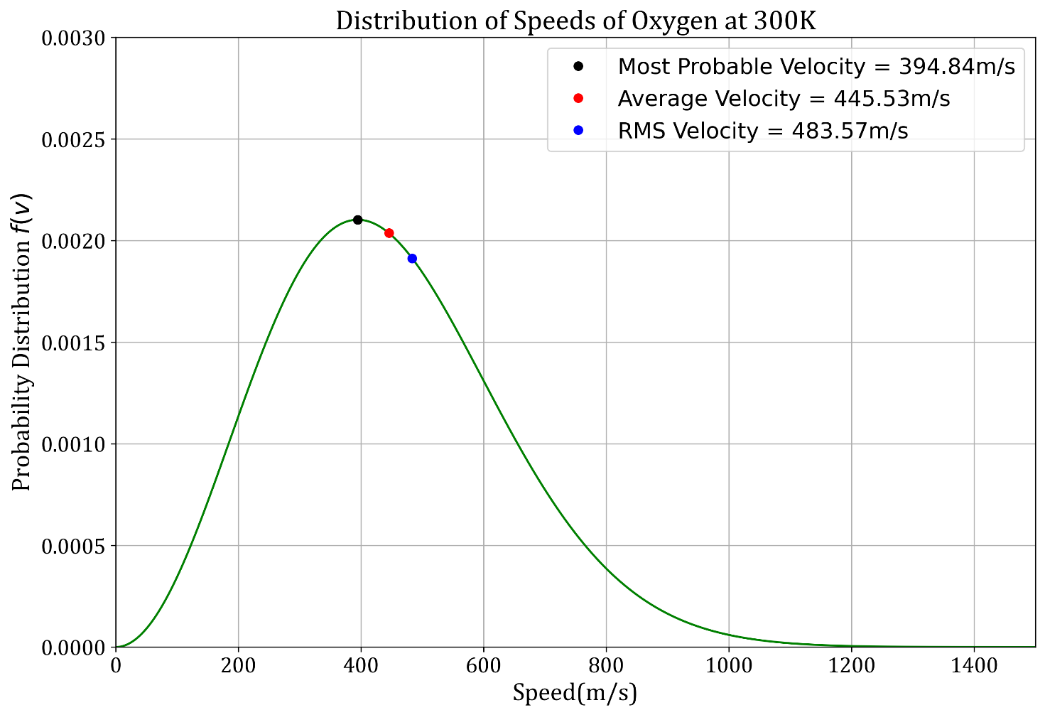
Observations and Conclusions:
- M-B distribution is a bell-shaped curve.
- As is evident from the curve, very small number of particles have very small and very large speeds.
- Most probable speed is the speed at which `f(v)` is maximum.
- It is clear that `v_(rms)>v_(avg)>v_(mp)`.
- That means number of particles moving at most probable speed is greater than the number of particles moving at mean speed.
- Also, `f(v_(mp))>f(v_(avg))>f(v_(rms))`.
Plotting Maxwell-Boltzmann speed distribution function for different gases: As is clear from the expression for f(v), the distribution of velocities depends on the mass of the molecules. Hence we shall now plot the probability distribution for different common gases at room temperature, that is, at 300 K. The python code to plot f(v) is given below.
Program in Python
===================================================================================
Program to plot Maxwell-Boltzmann speed distribution function for different gases
LANGUAGE :: PYTHON
Program By:: G.R. Mohanty , www.numericalmethods.in
===================================================================================
import matplotlib.pyplot as plt
import numpy as np

def mb_distribution(v, m):
    m = m/1000           #converting mass in grams to kilograms
    T = 300.00           #Temperature in Kelvins
    R = 8.31446261815324 # Universal Gas constant in units of J / (mol * K)
    return(4.0*np.pi*(v**2)*((m/(2*np.pi*R*T))**1.5)* np.exp(-(m*v**2)/(2*R*T)))

#colors[] is the array with the colors in which the plots are to be rendered
colors = ['crimson', 'orange', 'green', 'blue', 'purple', 'magenta']
plt.figure(figsize=(12, 8), dpi=300)
v = np.linspace(0, 3000, 1000)   # Velocities
plt.plot(v, mb_distribution(v, 2.016), colors[0], label=r'H$_2$') #Hydrogen
plt.plot(v, mb_distribution(v, 4.000), colors[1], label=r'He')    #Helium
plt.plot(v, mb_distribution(v, 20.18), colors[2], label=r'Ne')    #Neon
plt.plot(v, mb_distribution(v, 32.00), colors[3], label=r'O$_2$') #Oxygen
plt.plot(v, mb_distribution(v, 70.90), colors[4], label=r'Cl$_2$')#Chlorine
plt.plot(v, mb_distribution(v, 131.3), colors[5], label=r'Xe')    #Xenon

plt.xlabel(r'Speed(m/s)', font="Cambria", fontsize=18 )
plt.ylabel(r'Probability Distribution $f(v)$', font="Cambria", fontsize=18)
plt.xlim(0, 3000)
plt.xticks(font="Cambria", fontsize=16)
plt.yticks(font="Cambria", fontsize=16)
plt.title('Distribution of Speeds of Common Gases at 300 K', font="Cambria", fontsize=20)
plt.legend(title='Gas', fontsize=18)
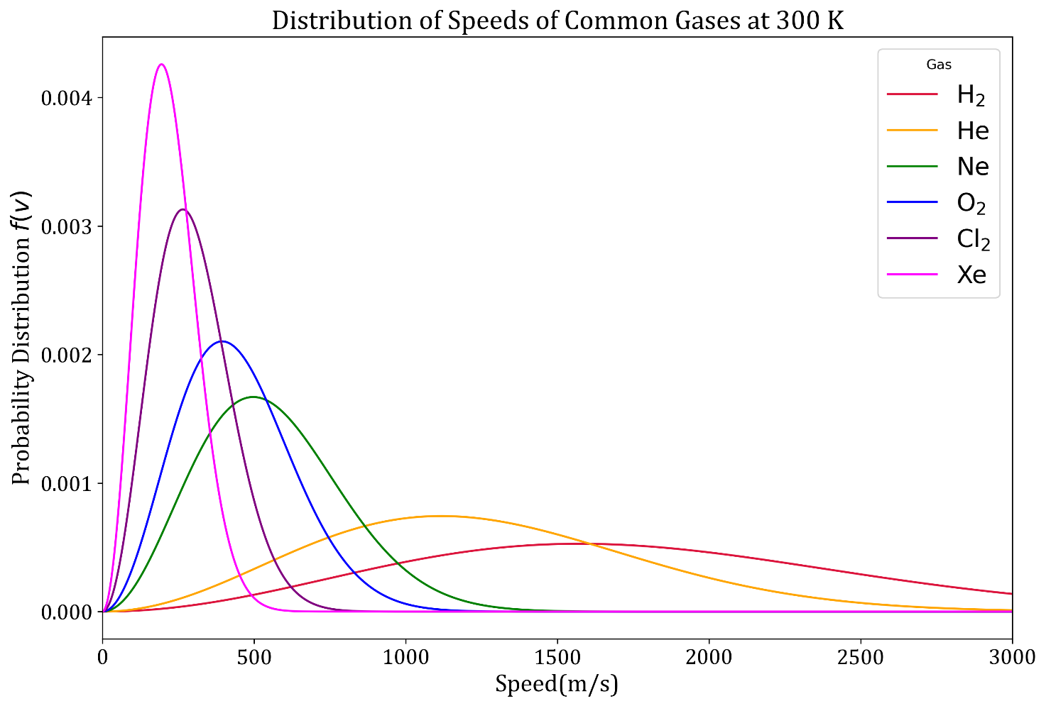
Observations and Conclusions:
- With increase in molecular mass (also molar mass), the peak of the curve shifts left.
- This implies that the heavier gases have lower `v_(mp),v_(avg) and v_(rms)` at any given temperature. In other words, molecules of lighter gases are faster.
- It can also be seen that for heavier gases the curve has higher and narrower peaks.
- For lighter gases the shape of the curve is more flat.
- From the above observations we can conclude that speeds of molecules of heavier gases vary within a narrower range than those for lighter gases.
- Probability of finding a Xe atom moving at its `v_(mp)` is far greater than the probability of finding a He atom moving at its `v_(mp)`.
Plotting Maxwell-Boltzmann speed distribution function at different temperatures: As we have plotted the velocity distribution of various gases at a common temperature, we can also plot the distribution for a given gas at different temperatures as demonstrated in the following code.
Program in Python
=======================================================================================
Program to plot Maxwell-Boltzmann speed distribution function at different temperatures
LANGUAGE :: PYTHON
Program By:: G.R. Mohanty , www.numericalmethods.in
=======================================================================================
import matplotlib.pyplot as plt
import numpy as np

def mb_distribution(v, m, T):
    m = m/1000           #converting mass in grams to kilograms
    R = 8.31446261815324 # Universal Gas constant in units of J / (mol * K)
    return(4.0*np.pi*(v**2)*((m/(2*np.pi*R*T))**1.5)* np.exp(-(m*v**2)/(2*R*T)))

#colors[] is the array with the colors in which the plots are to be rendered
colors = ['crimson', 'orange', 'green', 'blue', 'purple', 'magenta']
plt.figure(figsize=(12, 8), dpi=300)
v = np.linspace(0, 3000, 1000)   # Velocities

#Plotting velocity distribution of Oxygen at 10,250,500,1000,2000 and 5000 K
#molar mass of O2 is 32 grams

plt.plot(v, mb_distribution(v, 32.0,  50), colors[0], label='T=  10K')
plt.plot(v, mb_distribution(v, 32.0, 250), colors[1], label='T= 250K')
plt.plot(v, mb_distribution(v, 32.0, 500), colors[2], label='T= 500K')
plt.plot(v, mb_distribution(v, 32.0,1000), colors[3], label='T=1000K')
plt.plot(v, mb_distribution(v, 32.0,2000), colors[4], label='T=2000K')
plt.plot(v, mb_distribution(v, 32.0,5000), colors[5], label='T=5000K')

plt.xlabel(r'Speed(m/s)', font="Cambria", fontsize=18 )
plt.ylabel(r'Probability Distribution $f(v)$', font="Cambria", fontsize=18)
plt.xlim(0, 3000)
plt.xticks(font="Cambria", fontsize=16)
plt.yticks(font="Cambria", fontsize=16)
plt.title('Distribution of Speeds of Oxygen at Different Temperatures', font="Cambria", fontsize=20)
plt.legend(title='Temperatures', fontsize=16)
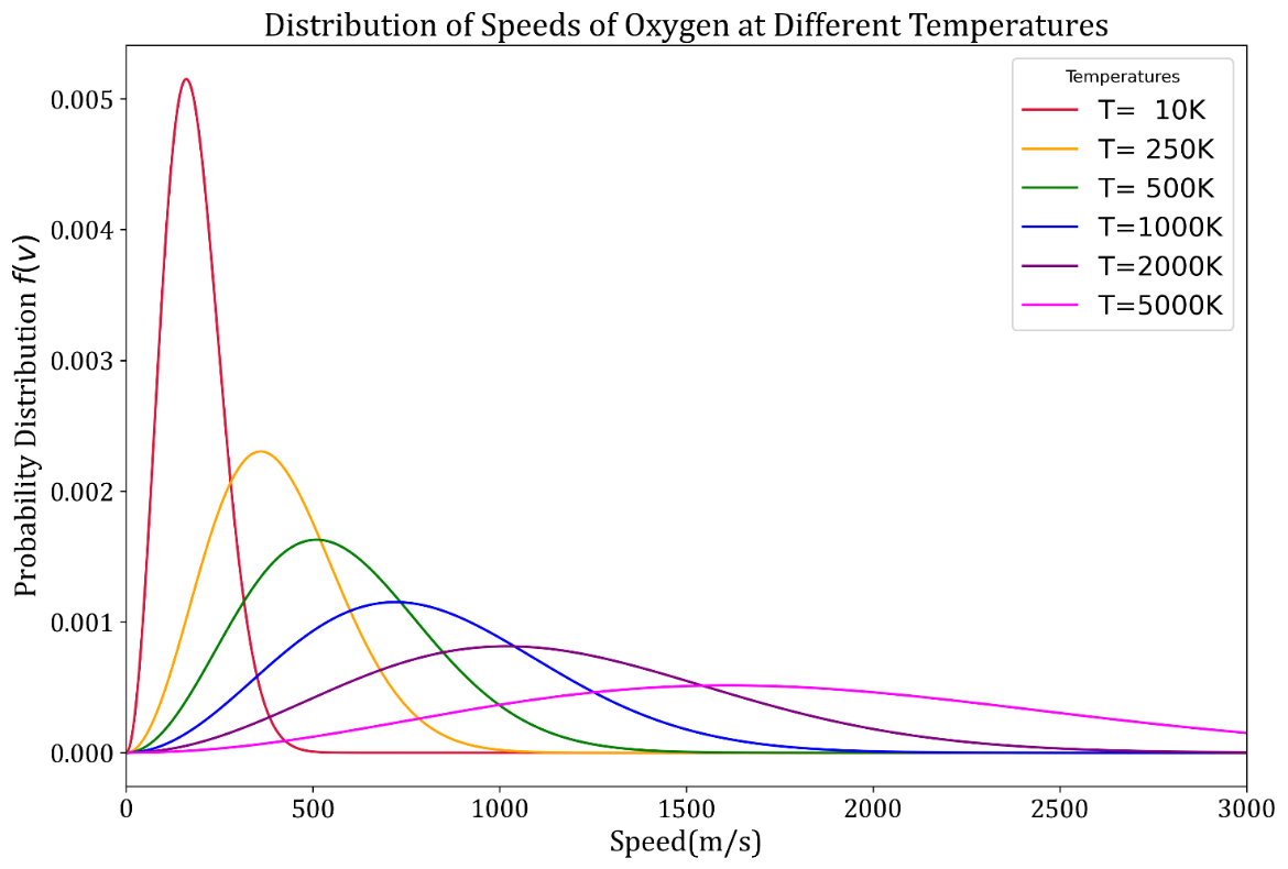
Observations and Conclusions:
- With increase in temperature, the peak of the curve shifts right.
- This implies that at higher temperature gases have higher `v_(mp),v_(avg) and v_(rms)` .
- With increase in temperature, the characteristics speeds of the molecules increase.
- It can also be seen that at lower temperatures the curves have higher and narrower peaks.
- At higher temperatures the shape of the curve is more flat.
- From the above observations we can conclude that speeds of molecules at lower temperatures vary within a narrower range than at higher temperatures.
- Probability of finding a molecule moving at its `v_(mp)` at lower temperature is far greater than the probability of finding it moving at its `v_(mp)` at a higher temperature.