A particle in a 1-D box (also called 1-D infinite potential well) experiences a potential given by:

`V(x)={(0, if a > x >0 text(,)), (infty, text( otherwise)):}`

After solving the time independent Schrodinger equation for this potential with appropriate boundary conditions we get the wave functions for such a particle.

`psi(x)={(sqrt(2/a)sin((npix)/a), text(for ) a > x >0),(0, text( otherwise)):}`.

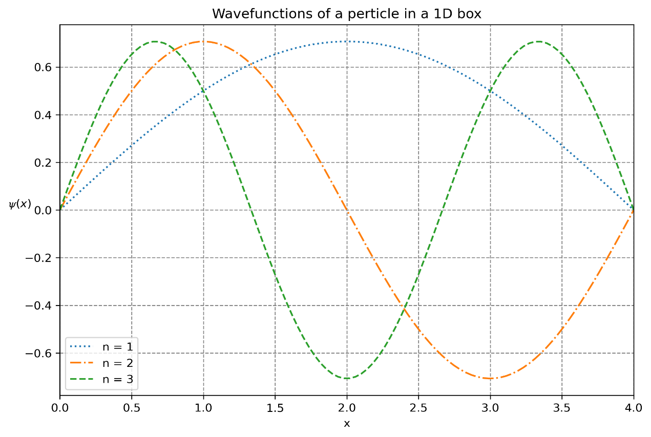
Here we plot these wave functions against the position coordinates `(x)` for n=1,2 and 3. The `ψ_n` are plotted only inside the box `(a>x>0)` as the wave functions vanish outside the box. For plotting, I have used the matplotlib library of PYTHON programming language. To write the code and render the plots I have used the SPYDER IDE. In the program given below we assume that the particle is confined between `x = 0` and `x = 2`, i.e, `a = 2` ( ‘a’ is the width of the box).

===================================================================================
Program to plot the wave functions of a particle in a 1-D Box  
LANGUAGE :: PYTHON 
Program By:: G.R. Mohanty , www.numericalmethods.in
===================================================================================
import matplotlib.pyplot as plt
import numpy as np

def wavefunction(a,n,x):
return (np.sqrt(2/a) * np.sin(n*np.pi*x/a))  #wavefunction 

plt.figure(figsize=(9,6), dpi=300)

a = 4     # 'a' is taken as the width of the box
x = np.linspace(0,a,100)

# the styles in which the plots are to be drawn
styles = [':','-.','--']  

# Plotting the wave functions for n = 1 to 3
for i in range(1,4):
plt.plot(x,wavefunction(a,i,x),styles[i-1], label='n = '+str(i))


plt.xlim(0,a)
plt.xlabel('x')
plt.ylabel('$\mathcal{\psi}(x)$',rotation='horizontal')
plt.title("Wavefunctions of a perticle in a 1D box")
plt.grid(color='gray',linestyle="--")
plt.legend()

Observations and Conclusions:

1. The wave functions vanish `(ψ_n=0)` at the boundaries, i.e., at `x=0` and `x=a` (in the program, a=4) where potential becomes infinite. Hence, we can say that the wave functions are continuous at the boundaries as outside the box `ψ_n = 0`.
2. The wave functions are either symmetric (even) or anti-symmetric (odd) with respect to the centre of the potential well. The wave functions with odd ‘n’ such as `ψ_1,(ψ_3 )` ̇etc. are even and those with even ‘n’ are odd with respect to the centre of the well.
3. As ‘n’ increases, each wave function has one more node than the previous one. Node is a point at which the wave function crosses the X-axis between origin and ‘a’.
4. It can be noted that `ψ_1` has no nodes, `ψ_2` bhas one node and so on. Hence `ψ_n` has `(n-1)` node.